15 Lines of Python: Poisson’s Equation in N Dimensions¶

Use Python magic to solve the Poisson equation in any number of dimensions

Physics¶

15 Lines of Python: Poisson’s Equation in N Dimensions¶

Use Python magic to solve the Poisson equation in any number of dimensions¶

No matter if you want to calculate heat conduction, the electrostatic or gravitational potential: it’s always the Poisson equation in one form or the other that you have to solve. Due to its importance, you will find a lot of resources on the internet showing you how to solve the Poisson equation numerically. Typically, they show you how to do it in one dimension or in two. Maybe in three. But have you ever seen how to write code that can solve it in an arbitrary number of dimensions? Probably not. This is what this article is about. We will use Python’s magic to solve the problem in a compact and high-performing way.

The basic solution scheme¶

The Poisson equation reads

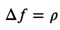
where 𝑓 and 𝜌 are real-valued functions of 𝑁 variables and Δ is the 𝑁-dimensional Laplace operator. For instance, for 𝑁=3 dimensions, we have

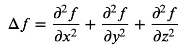
We still need to supply boundary conditions. So for concreteness, we say that we know the function values on the boundary. The easiest (though not fastest!) way to solve the Poisson equation numerically is using the Jacobi method. Basically, you discretize the functions, so that you only consider the functions on a grid of equidistant points. The partial derivatives are then replaced by finite differences and you end up (for 3 dimensions) with

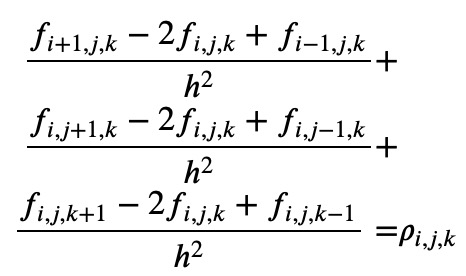
where 𝑓_𝑖,𝑗,𝑘 is the function value at the grid point with indices (𝑖,𝑗,𝑘) and ℎ is the spacing between two neighboring grid points. In the Jacobi method, you simply solve this algebraic equation for 𝑓_𝑖,𝑗,𝑘 and use that as an iteration scheme:

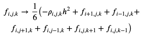
For 𝑁 different from 3, you get similar expressions with a different number of indices, of course. For 𝑁=2 we would have

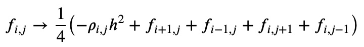
You probably get the idea. How can we generalize the approach for 𝑁 dimensions and write it in Python code without getting verbose or making compromises in terms of speed? Well, the crucial point is that on the right-hand side, you have a sum over all direct neighbors of the grid point in question. So we need to find a way how to enumerate the nearest grid points for any number of dimensions. I’ll give the solution first and discuss it then in detail.

The implementation for arbitrary dimensions¶

The solver contains two functions, a “driver” to control the iterations, and a “stepper” to do a single iteration. The driver is easy. It can be written like that:

Embedded content — see original: https://medium.com/@mathcube7/15-lines-of-python-the-poisson-equation-in-n-dimensions-ba0c8e186f92

Here we just apply the stepper repetitively until our result doesn’t change noticeably anymore (absolute toleranceatol). If this breaking condition is reached, we return the solution. Otherwise, if the maximum number of steps is exceeded, None is returned. f and rho can be NumPy arrays with any number of dimensions.

The actual work is done in the stepper function which is passed as argument to the solver. This allows us to easily replace it with some other stepping scheme later, if necessary. In our case, we implement the Jacobi stepper. The tricky part is “only” to enumerate the neighbors in an arbitrary number of dimensions. In fact, in Python, it can be written very compactly. Here is my solution:

Embedded content — see original: https://medium.com/@mathcube7/15-lines-of-python-the-poisson-equation-in-n-dimensions-ba0c8e186f92

The most salient point is the appearance of the slice object. This is a Python built-in object that most developers probably never have used before. In fact, whenever you use a Python slicing expression like f[3:10], for the Python interpreter this is just short-hand for f[slice(3, 10)]. Similarly, if you say f[3:], this is equivalent to f[slice(3, None)]. While the explicit use of slice objects is cumbersome in normal circumstances, it comes in handy if you want to take multi-dimensional slices. Maybe it's easier to see what's going on if we take a concrete example. In 2D, the Jacobi step in normal notation would look roughly like this:

Embedded content — see original: https://medium.com/@mathcube7/15-lines-of-python-the-poisson-equation-in-n-dimensions-ba0c8e186f92

which translates to

Embedded content — see original: https://medium.com/@mathcube7/15-lines-of-python-the-poisson-equation-in-n-dimensions-ba0c8e186f92

Note that in the array brackets, we have 2-tuples of slices! The idea of the jacobifunction listed above is just to build up those tuples of slices dynamically. For 𝑁-dimensional arrays, we have 𝑁-tuples of slices. Actually, it’s quite simple. You just have to know about the existence of the slice object in Python. The rest is straight forward. Having defined some 𝑁-dimensional arrays f and rho on a grid spacing h, you can then simply call

solve(f, rho, h, jacobi)

and it gives you the solution.

If you liked this article, you may want to consider becoming a Medium member to get unlimited access to all Medium articles. By registering using this link you can even support me as a writer.